import torch
import torch.nn as nn
import matplotlib.pyplot as plt
import numpy as np
import math
from IPython.display import display, clear_outputSimple ML Architectures to Solve the Heat Equation
Partial Differential Equations
Machine Learning
We use a neural network and polynomial regression to solve the heat equation and compare the results qualitatively.
I decided to try messing with the heat equation in my exploration of using ML to solve PDEs (and take a break from the Poisson equation). The equation itself is simple, as are the architectures I use to solve the equation, but this experiment proved interesting nonetheless. In particular, I found that the accuracy of the solution had more to do with the number and quality of the features I included for input than the architecture itself. I’ll elaborate upon what I mean below.
Heat Equation
I was motivated to solve the heat equation partially because of the nice visualizations that arise from a solution. I include an animation at the end of each solution I describe below. Unfortunately it can only run if the cell is executed; I’m having some environmental issues generating animations that play in-browser that I’ll troubleshoot later. Here’s the rendition of the heat equation I consider:
\[ \begin{alignat*}{2} & u_t(x,y,t)=\Delta_{(x,y)} u(x,y,t) && (x,y)\in B_1(0), t>0\\ & u(x,y,t)=0 && (x,y)\in\partial B_1(0), t\geq 0\\ & u(x,y,0)=\exp\left(-\frac{1}{1-(x^2+y^2)}\right) && (x,y)\in B_1(0) \end{alignat*} \]
for \(B_1(0)\subset\mathbb{R}^2\). The bump function makes for a particularly nice set of solutions to illustrate. The solution decays quickly, so we will only simulate it for a small period of time.
Simple Neural Network Solution
First, I will use a simple neural network with a single hidden layer. It doesn’t need to be very wide to get pretty good convergence to the solution. Here’s the architecture I use:
class NeuralNetwork(nn.Module):
    def __init__(self):
        super().__init__()
        self.sequential_model = nn.Sequential(
            nn.Linear(3, 8),
            nn.Sigmoid(),
            nn.Linear(8, 1)
        )

    def forward(self, x):
        return self.sequential_model(x)
Below is my data sampler function, simililar to the data sampler I used in my post on the Poisson equation. I sample 10000 points in my example and proceed to solve the equation for \(t\in\left[0,0.09\right]\).
def SampleFromUnitBall(points):
    d = torch.distributions.Uniform(-1,1)
    d_t = torch.distributions.Uniform(0,0.1)

    x = torch.Tensor(points,1)
    y = torch.Tensor(points,1)
    t = torch.Tensor(points,1)
    j=0
    k=0

    while j<points:
        x_temp = d.sample()
        y_temp = d.sample()
        t_temp = d_t.sample()
        if x_temp**2+y_temp**2<1 and t_temp!=0:
            x[j,0]=x_temp
            y[j,0]=y_temp
            t[j,0]=k*1/(10*points)
            j+=1
            if j%1000==0 and j!=0:
                k+=1000

    xbdry = torch.Tensor(points,1)
    ybdry = torch.Tensor(points,1)
    tbdry = torch.zeros(x.size(0)).unsqueeze(1)
    j=0

    while j<points:
        x_temp = d.sample()
        xbdry[j,0]=x_temp
        if j%2==0:
            ybdry[j,0]=math.sqrt(1-x_temp**2)
        else:
            ybdry[j,0]=-math.sqrt(1-x_temp**2)
        j+=1

    return x, y, t, xbdry, ybdry, tbdry
x, y, t, xbdry, ybdry, tbdry = SampleFromUnitBall(10000)The loss function is very similar to what we used in our Poisson solver. Again, I use a discrete mean-squared error function to compute the loss. In this case, I want to minimize the following,
\[L(x_{\text{int}},y_\text{int}, x_{\text{bdry}},y_{\text{bdry}}, t_{>0}):=\frac{1}{N_{\text{int}}}\sum_{j=1}^{N_{\text{int}}}|\Delta u(x^{(j)}_{\text{int}},y^{(j)}_{\text{int}}, t^{(j)}_{>0})-u(x^{(j)}_{\text{int}},y^{(j)}_{\text{int}}, t^{(j)}_{>0})|^2 \] \[ +\frac{1}{N_{\text{bdry}}}\sum_{j=1}^{N_{\text{bdry}}}|u(x^{(j)}_{\text{bdry}},y^{(j)}_{\text{bdry}},t^{(j)}_{>0})|^2+\frac{1}{N_{\text{int}}}\sum_{j=1}^{N_{\text{int}}}|u(x^{(j)}_{\text{int}},y^{(j)}_{\text{int}},0)-g(x^{(j)}_{\text{int}},y^{(j)}_{\text{int}})|^2 \]
where \(g(x,y):=\exp\left(-\frac{1}{1-(x^2+y^2)}\right)\).
To implement this loss function, I use the following code:
def g(x,y):
    return torch.exp(-1/(1-(x**2+y**2)))
def loss(x, y, t, xbdry, ybdry, tbdry, network):
x.requires_grad = True
y.requires_grad = True
t.requires_grad = True
temp_input = torch.cat((x,y,t),1)
w=network(temp_input)
temp_input_init = torch.cat((x,y,tbdry),1)
w_init = network(temp_input_init)
wbdry = network(torch.cat((xbdry, ybdry, t),1))
dw_dx = torch.autograd.grad(w.sum(), x, create_graph = True)[0]
ddw_ddx = torch.autograd.grad(dw_dx.sum(), x, create_graph = True)[0]
dw_dy = torch.autograd.grad(w.sum(), y, create_graph = True)[0]
ddw_ddy = torch.autograd.grad(dw_dy.sum(), y, create_graph = True)[0]
dw_dt = torch.autograd.grad(w.sum(), t, create_graph = True)[0]
A = torch.mean((dw_dt - (ddw_ddx+ddw_ddy))**2)
B = torch.mean((w_init-g(x,y))**2)
C = torch.mean((wbdry)**2)
return A+B+CNow I train the network. I use 100000 epochs to get pretty good convergence.
model = NeuralNetwork()
optimizer = torch.optim.SGD(model.parameters(), lr=0.01, momentum=.9)
epochs = 100000
loss_values = np.zeros(100000)
for i in range(epochs):
l = loss(x, y, t, xbdry, ybdry, tbdry, model)
l.backward()
optimizer.step()
optimizer.zero_grad()
loss_values[i]=l
if i%1000==0:
print("Loss at epoch {}: {}".format(i, l.item()))Loss at epoch 0: 0.2738669812679291
Loss at epoch 1000: 0.025970257818698883
Loss at epoch 2000: 0.02568979375064373
Loss at epoch 3000: 0.025230783969163895
Loss at epoch 4000: 0.024398991838097572
Loss at epoch 5000: 0.022912777960300446
Loss at epoch 6000: 0.02087295800447464
Loss at epoch 7000: 0.018625637516379356
Loss at epoch 8000: 0.015907008200883865
Loss at epoch 9000: 0.013540136627852917
Loss at epoch 10000: 0.012002145871520042
Loss at epoch 11000: 0.010946547612547874
Loss at epoch 12000: 0.01010743249207735
Loss at epoch 13000: 0.0094174575060606
Loss at epoch 14000: 0.008831574581563473
Loss at epoch 15000: 0.008312895894050598
Loss at epoch 16000: 0.007835050113499165
Loss at epoch 17000: 0.0073796845972537994
Loss at epoch 18000: 0.00693441741168499
Loss at epoch 19000: 0.006492464803159237
Loss at epoch 20000: 0.006053541321307421
Loss at epoch 21000: 0.0056252810172736645
Loss at epoch 22000: 0.0052236150950193405
Loss at epoch 23000: 0.004869983531534672
Loss at epoch 24000: 0.004583843518048525
Loss at epoch 25000: 0.004373359493911266
Loss at epoch 26000: 0.004231602419167757
Loss at epoch 27000: 0.004141609184443951
Loss at epoch 28000: 0.004085080698132515
Loss at epoch 29000: 0.004047917202115059
Loss at epoch 30000: 0.004021293483674526
Loss at epoch 31000: 0.00400038855150342
Loss at epoch 32000: 0.003982786554843187
Loss at epoch 33000: 0.0039673191495239735
Loss at epoch 34000: 0.003953419625759125
Loss at epoch 35000: 0.00394078902900219
Loss at epoch 36000: 0.003929249942302704
Loss at epoch 37000: 0.003918683156371117
Loss at epoch 38000: 0.003908993676304817
Loss at epoch 39000: 0.0039000948891043663
Loss at epoch 40000: 0.003891912754625082
Loss at epoch 41000: 0.0038843746297061443
Loss at epoch 42000: 0.0038774253334850073
Loss at epoch 43000: 0.0038710092194378376
Loss at epoch 44000: 0.0038650608621537685
Loss at epoch 45000: 0.003859535790979862
Loss at epoch 46000: 0.003854390000924468
Loss at epoch 47000: 0.003849589265882969
Loss at epoch 48000: 0.00384509633295238
Loss at epoch 49000: 0.0038408783730119467
Loss at epoch 50000: 0.0038368944078683853
Loss at epoch 51000: 0.0038331307005137205
Loss at epoch 52000: 0.0038295662961900234
Loss at epoch 53000: 0.003826176282018423
Loss at epoch 54000: 0.0038229411002248526
Loss at epoch 55000: 0.003819849109277129
Loss at epoch 56000: 0.0038168805185705423
Loss at epoch 57000: 0.0038140309043228626
Loss at epoch 58000: 0.0038112876936793327
Loss at epoch 59000: 0.0038086404092609882
Loss at epoch 60000: 0.0038060781080275774
Loss at epoch 61000: 0.003803590778261423
Loss at epoch 62000: 0.003801171202212572
Loss at epoch 63000: 0.0037988254334777594
Loss at epoch 64000: 0.0037965471856296062
Loss at epoch 65000: 0.003794319462031126
Loss at epoch 66000: 0.0037921415641903877
Loss at epoch 67000: 0.0037900148890912533
Loss at epoch 68000: 0.003787929890677333
Loss at epoch 69000: 0.003785883542150259
Loss at epoch 70000: 0.003783881664276123
Loss at epoch 71000: 0.003781920066103339
Loss at epoch 72000: 0.0037799954880028963
Loss at epoch 73000: 0.0037781083956360817
Loss at epoch 74000: 0.003776250407099724
Loss at epoch 75000: 0.00377441942691803
Loss at epoch 76000: 0.0037726142909377813
Loss at epoch 77000: 0.0037708329036831856
Loss at epoch 78000: 0.0037690771277993917
Loss at epoch 79000: 0.003767352784052491
Loss at epoch 80000: 0.003765658475458622
Loss at epoch 81000: 0.003763986984267831
Loss at epoch 82000: 0.0037623357493430376
Loss at epoch 83000: 0.0037607017438858747
Loss at epoch 84000: 0.003759087296202779
Loss at epoch 85000: 0.0037574912421405315
Loss at epoch 86000: 0.003755920333787799
Loss at epoch 87000: 0.0037543680518865585
Loss at epoch 88000: 0.0037528336979448795
Loss at epoch 89000: 0.0037513161078095436
Loss at epoch 90000: 0.0037498222663998604
Loss at epoch 91000: 0.0037483531050384045
Loss at epoch 92000: 0.0037469009403139353
Loss at epoch 93000: 0.0037454627454280853
Loss at epoch 94000: 0.003744041081517935
Loss at epoch 95000: 0.003742641070857644
Loss at epoch 96000: 0.0037412564270198345
Loss at epoch 97000: 0.003739887848496437
Loss at epoch 98000: 0.0037385355681180954
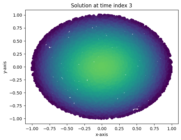
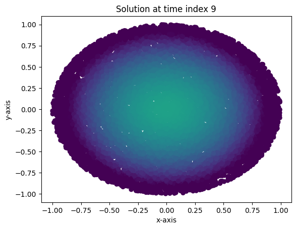
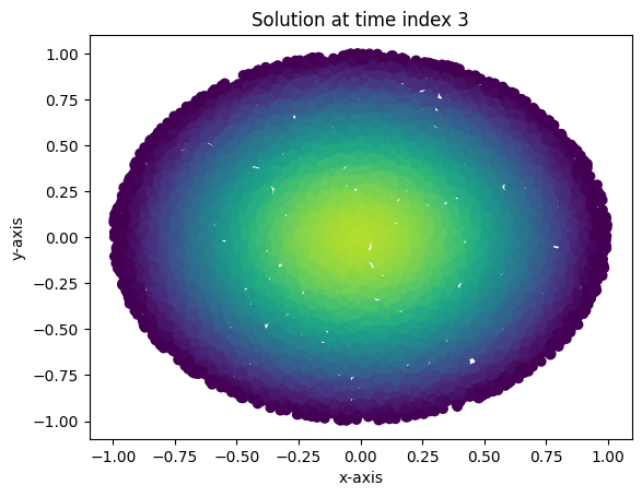
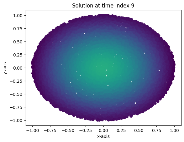
Loss at epoch 99000: 0.003737200517207384Evidently, one doesn’t need many input features, nor does one need a very wide network to get pretty good convergence. Moreover, I demonstrate the heat flow in the unit circle using the following plots and animation. Here, I’ve plotted a few instances of the solution over test data and three points in time in \(\left[0,0.09\right]\). Brighter colored scatter points indicate a higher value for \(u(x,y,t)\). As expected, the maximum value for \(u(x,y,t)\) decreases as time progresses, and the heat diffuses to be nearly constant.
x_test, y_test, z_test, xbdry_test, ybdry_test, zbdry_test = SampleFromUnitBall(10000)

def plot_points(time_index):
    with torch.no_grad():
        temp_input = torch.cat((x_test,y_test,torch.ones(10000).unsqueeze(1)*time_index/100),1)
        soln=model(temp_input)
    plt.scatter(x=x_test.detach(),y=y_test.detach(),c=soln.detach(), vmin=0, vmax=0.35)
    plt.title("Solution at time index " + str(time_index))
    plt.xlabel("x-axis")
    plt.ylabel("y-axis")
    plt.show()

plot_points(0)
plot_points(3)
plot_points(9)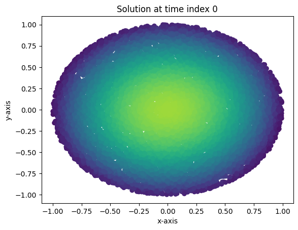
Running the cell below generates an animation of the solutions over time. I can even project the solutions past \(t=0.09\) to show that the heat diffusion is accurately captured past our sample times.
x_test, y_test, z_test, xbdry_test, ybdry_test, zbdry_test = SampleFromUnitBall(10000)
fig, ax = plt.subplots()
for k in range(20):
    with torch.no_grad():
        temp_input = torch.cat((x_test,y_test,torch.ones(10000).unsqueeze(1)*k/100),1)
        soln=model(temp_input)
    ax.cla()
    ax.scatter(x=x_test.detach(),y=y_test.detach(),c=soln.detach(), vmin=0, vmax=0.35)
    display(fig)
    clear_output(wait = True)
    plt.pause(0.1)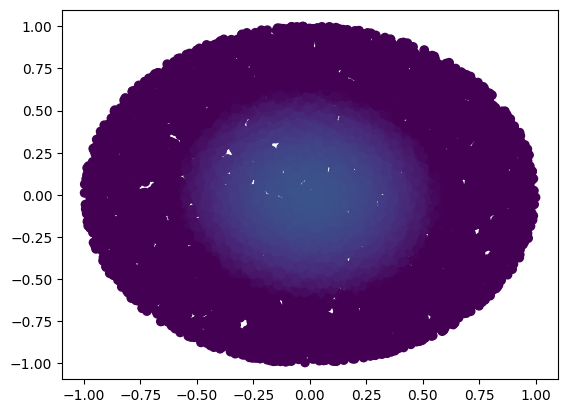
Polynomial regression solution
Now, I sample a new set of points and construct a “neural network” which actually allows me to run polynomial regression using my loss function. I show that a degree four polynomial in the input features is suitable for an accurate approximation to a solution of the problem. Here, I take advantage of the fact that the initial condition is radial in its input and admits a nice Taylor expansion in the radial coordinate \(r^2=x^2+y^2\). Hence, an accurate approximation of the initial condition may be obtained by using a low-degree polynomial. Interestingly, even though the Taylor series only contains even powers of \(r\), including all odd degree terms seemed to improve convergence. Furthermore, the polynomial approximation converges much more rapidly to the actual solution than the nueral network. Essentially, the polynomial approximation contains far more “useful” features than the simple coordinate and time input features I used in the neural network input.
x, y, t, xbdry, ybdry, tbdry = SampleFromUnitBall(10000)class NeuralNetwork2(nn.Module):
def __init__(self):
super().__init__()
self.sequential_model = nn.Sequential(
nn.Linear(32, 1)
)
def forward(self, x):
return self.sequential_model(x)The loss function is really ugly since I need to compute all polynomial features and their derivatives. I wanted to use scikit-learn’s polynomial feature class, but this destroyed the derivative data in my tensors, so I’d have to create a polynomial feature class from scratch. I might do this in the future, but for now everything is hardcoded.
def loss2(x, y, t, xbdry, ybdry, tbdry, network):
    x.requires_grad = True
    y.requires_grad = True
    t.requires_grad = True

    #Here come all of the polynomial features....

    x_2 = x**2
    y_2 = y**2
    x_3 = x**3
    y_3 = y**3
    x_4 = x**4
    y_4 = y**4
    xy_2 = x*(y**2)
    x_2y = (x**2)*y
    xyt = x*y*t
    x_2t = (x**2)*t
    y_2t = (y**2)*t
    t_3 = t**3
    t_4 = t**4
    x_3y = (x**3)*y
    xy_3 = x*(y**3)
    x_2y_2 = (x**2)*(y**2)
    x_3t = (x**3)*t
    x_2t_2 = (x**2)*(t**2)
    xt_3 = x*(t**3)
    y_3t = (y**3)*t
    y_2t_2 = (y**2)*(t**2)
    yt_3 = y*(t**3)
    xyt_2 = x*y*(t**2)
    xy_2t = x*(y**2)*t
    x_2yt = (x**2)*y*t
    xy = x*y
    t_2 = t**2
    xt = x*t
    yt = y*t
    xbdry_2 = xbdry**2
    ybdry_2 = ybdry**2
    xbdry_3 = xbdry**3
    ybdry_3 = ybdry**3
    xbdry_4 = xbdry**4
    ybdry_4 = ybdry**4
    xbdryybdry_2 = xbdry*(ybdry**2)
    xbdry_2ybdry = (xbdry**2)*ybdry
    xbdryybdryt = xbdry*ybdry*t
    xbdry_2t = (xbdry**2)*t
    ybdry_2t = (ybdry**2)*t
    xbdry_ybdry = xbdry*ybdry
    tbdry_2 = tbdry**2
    xbdry_t= xbdry*t
    ybdry_t = ybdry*t
    x_tbdry = x*tbdry
    y_tbdry = y*tbdry
    xytbdry = x*y*tbdry
    x_2tbdry = (x**2)*tbdry
    y_2tbdry = (y**2)*tbdry
    tbdry_3 = tbdry**3
    tbdry_4 = tbdry**4
    xbdry_3ybdry = (xbdry**3)*ybdry
    xbdryybdry_3 = xbdry*(ybdry**3)
    xbdry_2ybdry_2 = (xbdry**2)*(ybdry**2)
    xbdry_3t = (xbdry**3)*t
    xbdry_2t_2 = (xbdry**2)*(t**2)
    xbdryt_3 = xbdry*(t**3)
    ybdry_3t = (ybdry**3)*t
    ybdry_2t_2 = (ybdry**2)*(t**2)
    ybdryt_3 = ybdry*(t**3)
    x_3tbdry = (x**3)*tbdry
    x_2tbdry_2 = (x**2)*(tbdry**2)
    xtbdry_3 = x*(tbdry**3)
    y_3tbdry = (y**3)*tbdry
    y_2tbdry_2 = (y**2)*(tbdry**2)
    ytbdry_3 = y*(tbdry**3)
    xbdryybdryt_2 = xbdry*ybdry*(t**2)
    xbdryybdry_2t = xbdry*(ybdry**2)*t
    xbdry_2ybdryt = (xbdry**2)*ybdry*t
    xytbdry_2 = x*y*(tbdry**2)
    xy_2tbdry = x*(y**2)*tbdry
    x_2ytbdry = (x**2)*y*tbdry

    ##End of polynomial features

    temp_input = torch.cat((x,y,t,x_2,y_2,xy,t_2,xt,yt,x_4,y_4,t_4,x_3y,xy_3,x_2y_2,x_3t,x_2t_2,xt_3,y_3t,y_2t_2,yt_3,xyt_2,xy_2t,x_2yt,x_3,y_3,xy_2,x_2y,xyt,x_2t,y_2t,t_3),1)
    w=network(temp_input)
    temp_input_init = torch.cat((x,y,tbdry,x_2,y_2,xy,tbdry_2,x_tbdry,y_tbdry,x_4,y_4,tbdry_4,x_3y,xy_3,x_2y_2,x_3tbdry,x_2tbdry_2,xtbdry_3,y_3tbdry,y_2tbdry_2,ytbdry_3,xytbdry_2,xy_2tbdry,x_2ytbdry,x_3,y_3,xy_2,x_2y,xytbdry,x_2tbdry,y_2tbdry,tbdry_3),1)
    w_init = network(temp_input_init)
    wbdry = network(torch.cat((xbdry, ybdry, t,xbdry_2,ybdry_2,xbdry_ybdry,t_2,xbdry_t,ybdry_t,xbdry_4,ybdry_4,t_4,xbdry_3ybdry,xbdryybdry_3,xbdry_2ybdry_2,xbdry_3t,xbdry_2t_2,xbdryt_3,ybdry_3t,ybdry_2t_2,ybdryt_3,xbdryybdryt_2,xbdryybdry_2t,xbdry_2ybdryt,xbdry_3,ybdry_3,xbdryybdry_2,xbdry_2ybdry,xbdryybdryt,xbdry_2t,ybdry_2t,t_3),1))

    dw_dx = torch.autograd.grad(w.sum(), x, create_graph = True)[0]
    ddw_ddx = torch.autograd.grad(dw_dx.sum(), x, create_graph = True)[0]
    dw_dy = torch.autograd.grad(w.sum(), y, create_graph = True)[0]
    ddw_ddy = torch.autograd.grad(dw_dy.sum(), y, create_graph = True)[0]
    dw_dt = torch.autograd.grad(w.sum(), t, create_graph = True)[0]

    A = torch.mean((dw_dt - (ddw_ddx+ddw_ddy))**2)
    B = torch.mean((w_init-g(x,y))**2)
    C = torch.mean((wbdry)**2)
    #print("Loss for each item: {}, {}, {}".format(A,B,C))
    return A+B+C
Below, I define a helper function for computing values the network generates from input data. It computes all of the needed polynomial features before supplying them into the network.
def network_value(x, y, t, network):
    x_2 = x**2
    y_2 = y**2
    x_3 = x**3
    y_3 = y**3
    x_4 = x**4
    y_4 = y**4
    xy_2 = x*(y**2)
    x_2y = (x**2)*y
    xyt = x*y*t
    x_2t = (x**2)*t
    y_2t = (y**2)*t
    t_3 = t**3
    t_4 = t**4
    xy = x*y
    t_2 = t**2
    xt = x*t
    yt = y*t
    x_3y = (x**3)*y
    xy_3 = x*(y**3)
    x_2y_2 = (x**2)*(y**2)
    x_3t = (x**3)*t
    x_2t_2 = (x**2)*(t**2)
    xt_3 = x*(t**3)
    y_3t = (y**3)*t
    y_2t_2 = (y**2)*(t**2)
    yt_3 = y*(t**3)
    xyt_2 = x*y*(t**2)
    xy_2t = x*(y**2)*t
    x_2yt = (x**2)*y*t
    temp_input = torch.cat((x,y,t,x_2,y_2,xy,t_2,xt,yt,x_4,y_4,t_4,x_3y,xy_3,x_2y_2,x_3t,x_2t_2,xt_3,y_3t,y_2t_2,yt_3,xyt_2,xy_2t,x_2yt,x_3,y_3,xy_2,x_2y,xyt,x_2t,y_2t,t_3),1)
    w=network(temp_input)
    return w
Now, I build and train the network.
model2 = NeuralNetwork2()
optimizer2 = torch.optim.SGD(model2.parameters(), lr=0.01, momentum=.9)
epochs = 100000
loss_values = np.zeros(100000)
for i in range(epochs):
l = loss2(x, y, t, xbdry, ybdry, tbdry, model2)
l.backward()
optimizer2.step()
optimizer2.zero_grad()
loss_values[i]=l
if i%1000==0:
print("Loss at epoch {}: {}".format(i, l.item()))Loss at epoch 0: 0.89188551902771
Loss at epoch 1000: 0.003854417707771063
Loss at epoch 2000: 0.0035820240154862404
Loss at epoch 3000: 0.003396423067897558
Loss at epoch 4000: 0.0032313335686922073
Loss at epoch 5000: 0.003081361996009946
Loss at epoch 6000: 0.0029437472112476826
Loss at epoch 7000: 0.0028166514821350574
Loss at epoch 8000: 0.0026987330056726933
Loss at epoch 9000: 0.002588952425867319
Loss at epoch 10000: 0.002486460143700242
Loss at epoch 11000: 0.0023905490525066853
Loss at epoch 12000: 0.0023006070405244827
Loss at epoch 13000: 0.0022161088418215513
Loss at epoch 14000: 0.002136589726433158
Loss at epoch 15000: 0.0020616455003619194
Loss at epoch 16000: 0.0019909129478037357
Loss at epoch 17000: 0.001924069132655859
Loss at epoch 18000: 0.0018608317477628589
Loss at epoch 19000: 0.0018009372288361192
Loss at epoch 20000: 0.0017441592644900084
Loss at epoch 21000: 0.001690280856564641
Loss at epoch 22000: 0.0016391162062063813
Loss at epoch 23000: 0.0015904909232631326
Loss at epoch 24000: 0.0015442450530827045
Loss at epoch 25000: 0.0015002338914200664
Loss at epoch 26000: 0.0014583258889615536
Loss at epoch 27000: 0.0014183972962200642
Loss at epoch 28000: 0.0013803349575027823
Loss at epoch 29000: 0.0013440358452498913
Loss at epoch 30000: 0.0013093998422846198
Loss at epoch 31000: 0.0012763398699462414
Loss at epoch 32000: 0.0012447721092030406
Loss at epoch 33000: 0.0012146164663136005
Loss at epoch 34000: 0.0011857992503792048
Loss at epoch 35000: 0.0011582525912672281
Loss at epoch 36000: 0.0011319173499941826
Loss at epoch 37000: 0.0011067262385040522
Loss at epoch 38000: 0.001082623261027038
Loss at epoch 39000: 0.001059556845575571
Loss at epoch 40000: 0.0010374787962064147
Loss at epoch 41000: 0.0010163375409319997
Loss at epoch 42000: 0.000996090704575181
Loss at epoch 43000: 0.0009766991715878248
Loss at epoch 44000: 0.0009581181220710278
Loss at epoch 45000: 0.0009403128060512245
Loss at epoch 46000: 0.0009232479496859014
Loss at epoch 47000: 0.0009068892104551196
Loss at epoch 48000: 0.0008912016055546701
Loss at epoch 49000: 0.0008761570206843317
Loss at epoch 50000: 0.0008617275161668658
Loss at epoch 51000: 0.0008478870149701834
Loss at epoch 52000: 0.0008346029790118337
Loss at epoch 53000: 0.0008218575385399163
Loss at epoch 54000: 0.0008096238598227501
Loss at epoch 55000: 0.0007978778448887169
Loss at epoch 56000: 0.0007866068044677377
Loss at epoch 57000: 0.0007757834391668439
Loss at epoch 58000: 0.0007653866778127849
Loss at epoch 59000: 0.0007554012699984014
Loss at epoch 60000: 0.0007458093459717929
Loss at epoch 61000: 0.0007365943747572601
Loss at epoch 62000: 0.0007277417462319136
Loss at epoch 63000: 0.0007192345801740885
Loss at epoch 64000: 0.0007110605365596712
Loss at epoch 65000: 0.0007032029679976404
Loss at epoch 66000: 0.0006956501747481525
Loss at epoch 67000: 0.0006883873138576746
Loss at epoch 68000: 0.0006814048392698169
Loss at epoch 69000: 0.0006746951257809997
Loss at epoch 70000: 0.0006682390812784433
Loss at epoch 71000: 0.0006620289059355855
Loss at epoch 72000: 0.0006560610490851104
Loss at epoch 73000: 0.0006503157783299685
Loss at epoch 74000: 0.0006447912310250103
Loss at epoch 75000: 0.0006394768133759499
Loss at epoch 76000: 0.0006343616987578571
Loss at epoch 77000: 0.0006294394261203706
Loss at epoch 78000: 0.0006247067940421402
Loss at epoch 79000: 0.0006201465730555356
Loss at epoch 80000: 0.0006157630705274642
Loss at epoch 81000: 0.0006115416181273758
Loss at epoch 82000: 0.0006074761622585356
Loss at epoch 83000: 0.0006035627448000014
Loss at epoch 84000: 0.0005997983971610665
Loss at epoch 85000: 0.0005961735732853413
Loss at epoch 86000: 0.000592682627029717
Loss at epoch 87000: 0.000589318631682545
Loss at epoch 88000: 0.0005860833334736526
Loss at epoch 89000: 0.0005829664296470582
Loss at epoch 90000: 0.0005799678037874401
Loss at epoch 91000: 0.0005770765710622072
Loss at epoch 92000: 0.0005742927896790206
Loss at epoch 93000: 0.0005716124433092773
Loss at epoch 94000: 0.0005690286634489894
Loss at epoch 95000: 0.0005665384232997894
Loss at epoch 96000: 0.0005641438765451312
Loss at epoch 97000: 0.0005618334980681539
Loss at epoch 98000: 0.0005596067057922482
Loss at epoch 99000: 0.0005574636743403971Evidently, the convergence to a solution is much more rapid (one needs far fewer epochs to obtain the same loss as in the more traditional neural network). Below are plots of the solution, as well as an animation. These look virtually identical to the results using the more traditional neural network.
x_test, y_test, z_test, xbdry_test, ybdry_test, zbdry_test = SampleFromUnitBall(10000)

def plot_points2(time_index):
    with torch.no_grad():
        soln = network_value(x_test,y_test,torch.ones(10000).unsqueeze(1)*time_index/100,model2)
    plt.scatter(x=x_test.detach(),y=y_test.detach(),c=soln.detach(), vmin=0, vmax=0.35)
    plt.title("Solution at time index " + str(time_index))
    plt.xlabel("x-axis")
    plt.ylabel("y-axis")
    plt.show()

plot_points2(0)
plot_points2(3)
plot_points2(9)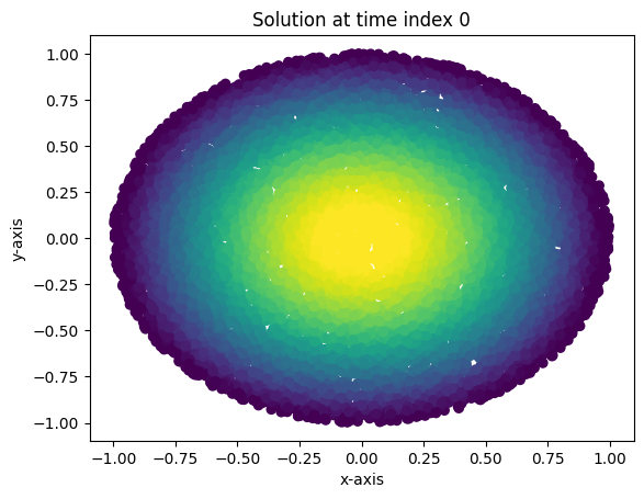
Interestingly, projecting the solution into the future past \(t=0.09\) seems to yield a less accurate solution than the one I got from the neural network. But still, this isn’t bad and leads to some interesting theoretical questions as to the degree of polynomial required to get “future in time” predictions which are as accurate as the network.
x_test, y_test, z_test, xbdry_test, ybdry_test, zbdry_test = SampleFromUnitBall(10000)
fig, ax = plt.subplots()
for k in range(20):
    with torch.no_grad():
        soln = network_value(x_test,y_test,torch.ones(10000).unsqueeze(1)*k/100,model2)
    ax.cla()
    ax.scatter(x=x_test.detach(),y=y_test.detach(),c=soln.detach(), vmin=0, vmax=0.35)
    display(fig)
    clear_output(wait = True)
    plt.pause(0.1)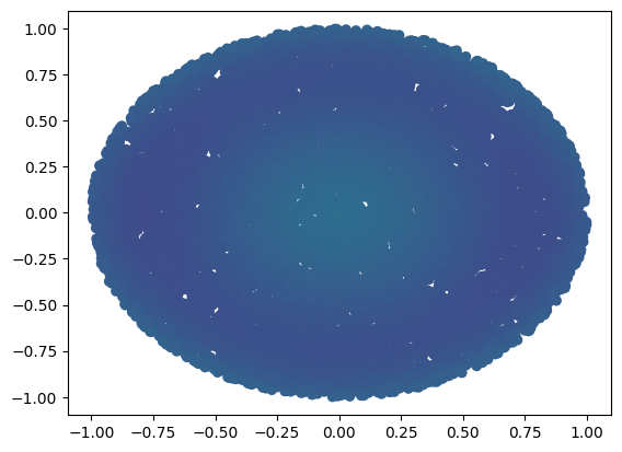
Now that I have all of this set up, it would be interesting to run the code against more complicated initial conditions. I leave this exercise to the reader. Next time, I think I’ll get back to something more like the Poisson equation, or perhaps work on solving PDEs which arise from variational problems. Overall, solving PDEs using neural networks or polynomial regression is proving productive and interesting!